Whole-Genome DNA Methylation data analysis pipeline

From sequencing data to differential methylation analysis

Jyotirmoy Das

Bioinformatics Unit, Core Facility, Faculty of Medicine and Health Sciences, Linköping University

Clinical Genomics Linköping, Linköping University


jyotirmoy.das@liu.se

cgl-240215.netlify.app

Features of Bioinformatics pipelines


  • A bioinformatics pipeline typically depends on the availability of several resources, including adequate storage, computer units, network connectivity, and appropriate software execution environment.

  • Automation helps manage bioinformatics resources and workflows and streamlines day-to-day bioinformatics operations.

  • Containers are a standard unit of software that enables the packaging of software and its dependencies to be run on different computers and operating systems with virtually no configuration changes.

  • Version control of the pipeline should include semantic versioning of the deployed instance of a pipeline as a whole.

  • The most critical requirement for implementing a bioinformatics pipeline is a proper, systematic clinical validation in the context of the entire next-generation sequencing (NGS) assay.

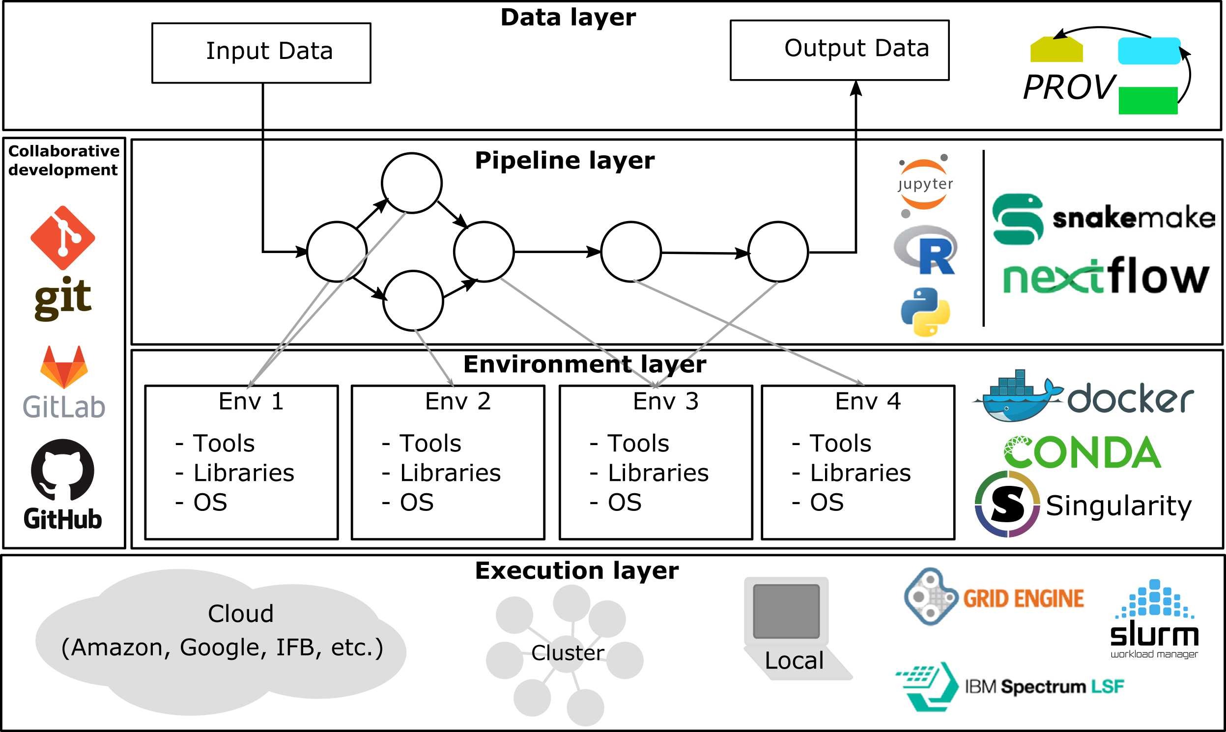
Landscape of a generic pipeline

Figure: Analysis can be defined with four layers: Data, pipeline, software environment, and execution layers.

Figure: Analysis can be defined with four layers: Data, pipeline, software environment, and execution layers.

Comprehensive DNA methylation data analysis pipelines

Curated from Gong T el al (2022)

Twist-suggested methylation data analysis flowchart
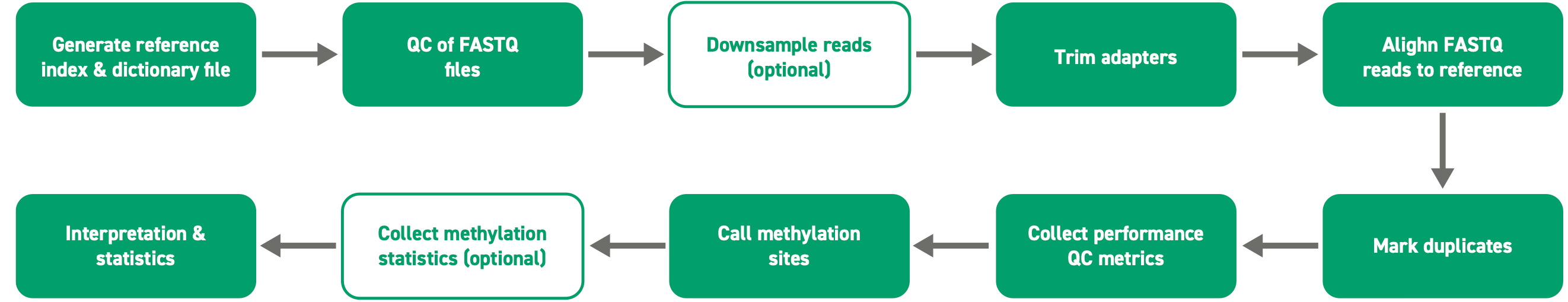
Figure: Twist Methylation Analysis Pipeline

Figure: Twist Methylation Analysis Pipeline


Optional steps:
- Downsampling reads (seqtk)
- Collect methylation stats


Important information
1. same pipeline can be used for Twist custom methylation panel
2. genome reference file should match the panel’s genome build
3. replace the Methylome V1 probe and target BED file.

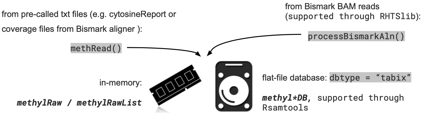
Tools for methylation data processing

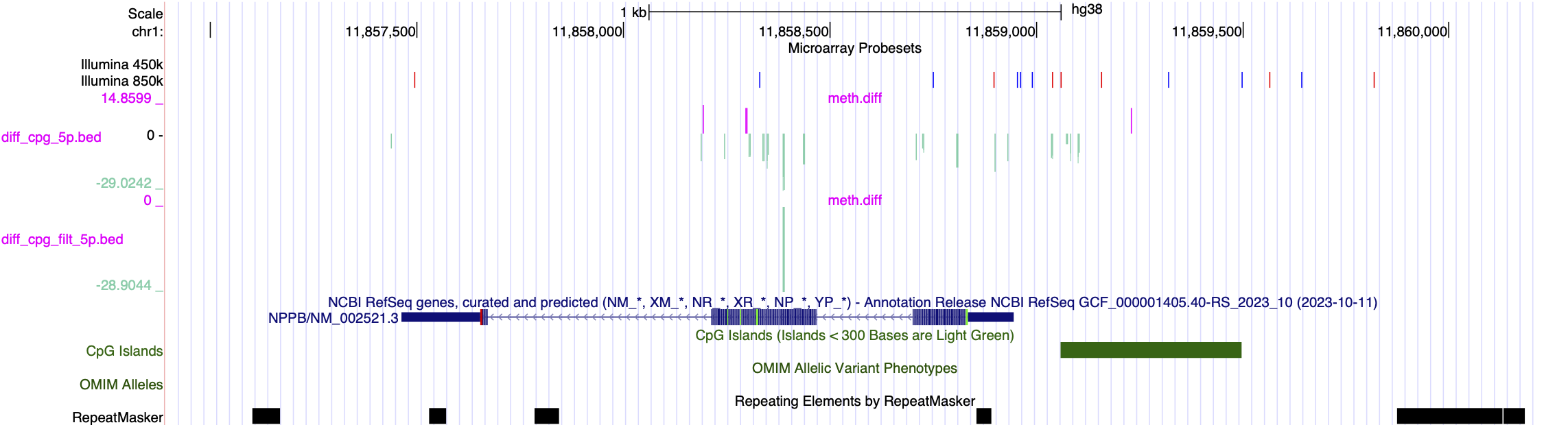
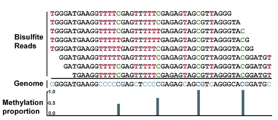
Some examples of methylation data analysis results

Genome Browser View showing region chr1:11,857,464-11,858,945 of the hg38 assembly. 1


Differential Methylation Analysis

A. MethylKit

%%{init: {"flowchart": {"htmlLabels": false}} }%%
flowchart TB
  id1["Reading methylation 
  calls from Bismark 
  alignments"] 
  id2["filtering on read 
  coverage"]

  id1 --> id2
  id2 --> id3[merging samples]
  id3 --> id4[[calculate DiffMeth]]
  id4 --> id5(Annotation)

B. EdgeR

%%{init: {"flowchart": {"htmlLabels": false}} }%%
flowchart TB
  id1["Reading coverage files
  from Bismark results"] 
  id2["counts, samples, 
  chromosome location"]
  id3["filtering chromosomes,
  finding nearest TSS,
  filter by coverage"]

  id1 --> id2
  id2 --> id3
  id3 --> id6[[Calculate M-value]]
  id6 --> id7[[Calculate diff meth]]

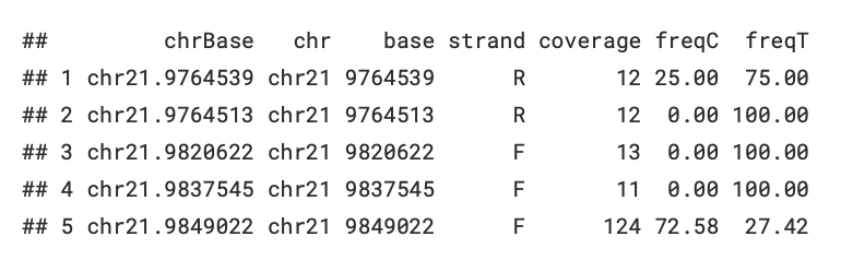
A1. MethylKit: Reading data

Methylation coverage data from bismark

Methylation coverage data from bismark

Bismark BAM reads

Bismark BAM reads

Reading files in MethylKit

Reading files in MethylKit

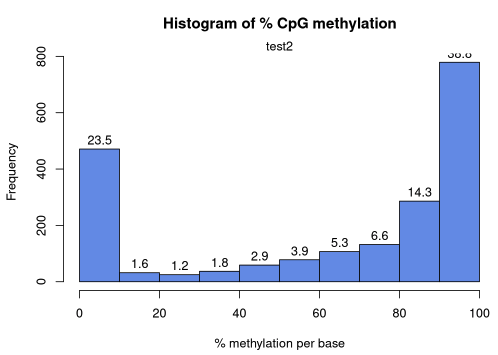
A2. MethylKit: Summarize statistics on samples

getMethylationStats(methylRaw) 


methylation statistics per base
summary:
    Min. 1st Qu.  Median    Mean 3rd Qu.    Max. 
    0.00   20.00   82.79   63.17   94.74  100.00 
percentiles:
       0%       10%       20%       30%       40%       50%       60%       70% 
  0.00000   0.00000   0.00000  48.38710  70.00000  82.78556  90.00000  93.33333 
      80%       90%       95%       99%     99.5%     99.9%      100% 
 96.42857 100.00000 100.00000 100.00000 100.00000 100.00000 100.00000
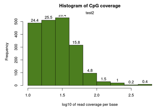


Histogram of % CpG methylaiton

Histogram of % CpG methylaiton

getCoverageStats(methylRaw)


read coverage statistics per base
summary:
    Min. 1st Qu.  Median    Mean 3rd Qu.    Max. 
    10.00  16.00   26.00   34.45   39.00  630.00 
percentiles:
       0%       10%       20%       30%       40%       50%       60%       70% 
    10.000    11.000    14.000    17.000   20.000    26.000    30.000    36.000 
      80%       90%       95%       99%     99.5%     99.9%      100% 
   42.000     60.000   78.750    195.800   328.300  441.945    630.000


Histogram of CpG coverage

Histogram of CpG coverage

A3. MethylKit: Compare Samples

get the bases covered in all samples: merge all samples to one object for base-pair locations that are covered in all samples:

assocComp - Batch Effect correction
tileMethylCounts - Tiling window analysis

unite(methylRawList) --> methylBase

getCorrelation(methylBase)

Samples correlation

Samples correlation

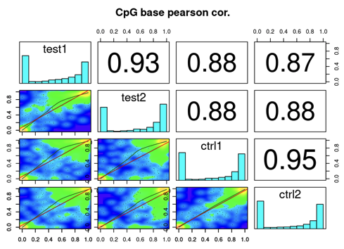
clusterSamples(methylBase)

Samples cluster

Samples cluster

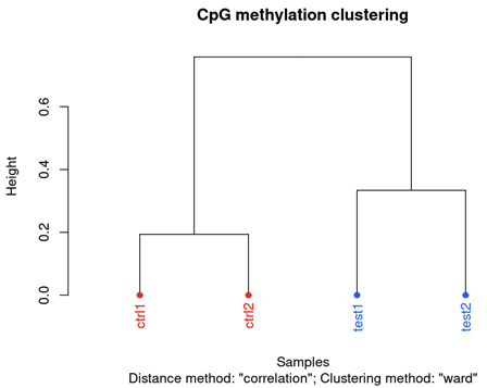
PCASamples(methylBase)

Samples PCA

Samples PCA

A4. MethylKit: Differential Analysis

Testing for differential methylation using either Fisher’s exact test or Chisq test for logistic regression model (depending on the sample size per set) with p-value adjustment using SLIM 1 method (Wang, Tuominen, and Tsai 2010) :

calculateDiffMeth(methylBase) → methylDiff


Optional correction for overdispersion if more variability present in the data than assumed by binomial distribution:

calculateDiffMeth(methylBase,overdispersion="MN")


Covariates can be included in the analysis to separate the influence of the covariates from the treatment effect via the logistic regression model.

covariates=data.frame(age=c(30,80,30,80))
calculateDiffMeth(methylBase,covariates=covariates)

getMethylDiff - filtering differential bases

calculateDiffMeth(...,
mc.cores=2) - use multiple cores

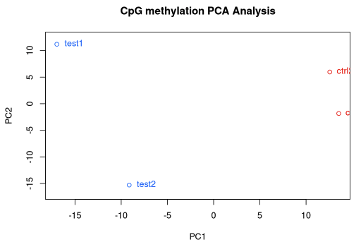
A5. MethylKit: Annotation

Use genomation package to annotate differentially methylated regions/bases based on gene annotation:
first read the gene BED file:

gene.obj=readTranscriptFeatures(system.file("extdata", "refseq.hg18.bed.txt",package = "methylKit"))


then get all differentially methylated bases:

myDiff25p=getMethylDiff(methylDiff,difference=25, qvalue=0.01)


now annotate differentially methylated CpGs with promoter/exon/intron using annotation data

diffAnn=annotateWithGeneParts(as(myDiff25p,"GRanges"), gene.obj)


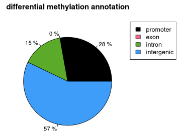
finally visualize the annotation:

plotTargetAnnotation(diffAnn,precedence=TRUE, main="differential methylation annotation")


differential methylation annotation

differential methylation annotation

B1. EdgeR: Reading Data

The EdgeR function readBismark2DGE reads all the files and collates the counts for all the sample into one data object:


> Sample <- row.names(targets)
> files <- paste0(Sample,".bismark.cov.gz")
> yall <- readBismark2DGE(files, sample.names=Sample)

Reading P6_1.bismark.cov.gz
Reading P6_4.bismark.cov.gz
Reading P7_2.bismark.cov.gz
Reading P7_5.bismark.cov.gz
Reading P8_3.bismark.cov.gz
Reading P8_6.bismark.cov.gz
Hashing ...
Collating counts ...

> dim(yall)

[1] 3538117      12
> head(yall$counts)

              P6_1-Me P6_1-Un P6_4-Me P6_4-Un P7_2-Me P7_2-Un P7_5-Me P7_5-Un
chr15-3051454      14       2      18       0       6       0      15       1
chr15-3051455       1       0       1       0       0       0       0       0
chr15-3051486      16       0      17       1       6       0      16       0
chr15-3051555      13       3      18       0       5       1      16       0
chr15-3051556       1       0       1       0       0       0       0       0
chr15-3051559      14       2      15       3       5       1      15       1
              P8_3-Me P8_3-Un P8_6-Me P8_6-Un
chr15-3051454       8       0       3       0
chr15-3051455       0       0       1       0
chr15-3051486       8       0       3       0
chr15-3051555       8       0       3       0
chr15-3051556       0       0       1       0
chr15-3051559       8       0       3       0
  • The EdgeR package stores the counts and associated annotation in a simple list-based data object called a “DGEList”.
  • There is a row for each CpG locus found in any of the files. There columns of methylated and unmethylated counts for each sample. The chromosomes and genomic loci are stored in the annotation data.frame.
  • Summary information on each sample is stored in yall$samples

B2. EdgeR: Filtering and Annotation

Filtering unassembled chromosomes


Sort into genomic order


Gene Annotation


Filtering to remove low counts

> TSS <- nearestTSS(yall$genes$Chr, yall$genes$Locus, species="Mm")
> yall$genes$EntrezID <- TSS$gene_id
> yall$genes$Symbol <- TSS$symbol
> yall$genes$Strand <- TSS$strand
> yall$genes$Distance <- TSS$distance
> yall$genes$Width <- TSS$width
> head(yall$genes)

              Chr   Locus EntrezID Symbol Strand Distance  Width
chr1-3020689 chr1 3020689   497097   Xkr4      -  -650809 457017
chr1-3020690 chr1 3020690   497097   Xkr4      -  -650808 457017
chr1-3020708 chr1 3020708   497097   Xkr4      -  -650790 457017
chr1-3020724 chr1 3020724   497097   Xkr4      -  -650774 457017
chr1-3020725 chr1 3020725   497097   Xkr4      -  -650773 457017
chr1-3020814 chr1 3020814   497097   Xkr4      -  -650684 457017


> Coverage <- yall$counts[, Methylation=="Me"] + yall$counts[, Methylation=="Un"]
> head(Coverage)

             P6_1-Me P6_4-Me P7_2-Me P7_5-Me P8_3-Me P8_6-Me
chr1-3020689      16      21       4      13       6       2
chr1-3020690      37      47      18      46      15      22
chr1-3020708       0       2       0       1       0       0
chr1-3020724      16      21       4      14       6       2
chr1-3020725      37      47      18      46      15      22
chr1-3020814       0       0       0       1       0       0

B3. EdgeR: Normalization


  • the methylated and unmethylated reads for the same sample are treated on the same scale, users need to set the library sizes to be equal for each pair of libraries.


  • the library sizes for each sample to be the average of the total read counts for the methylated and unmethylated libraries. 1
> TotalLibSize <- y$samples$lib.size[Methylation=="Me"] +
+                 y$samples$lib.size[Methylation=="Un"]
> y$samples$lib.size <- rep(TotalLibSize, each=2)
> y$samples
         
        group lib.size norm.factors
P6_1-Me    P6 27754786            1
P6_1-Un    P6 27754786            1
P6_4-Me    P7 41007143            1
P6_4-Un    P7 41007143            1
P7_2-Me    P8 21424225            1
P7_2-Un    P8 21424225            1
P7_5-Me    P6 26197143            1
P7_5-Un    P6 26197143            1
P8_3-Me    P7 18782105            1
P8_3-Un    P7 18782105            1
P8_6-Me    P8 15539660            1
P8_6-Un    P8 15539660            1

B4. EdgeR: Calculating differential methylation

Exploring differences between samples

In microarray methylation studies, a common measure of methylation level is the M-value, which is defined as \[ M = log_{2} \frac{(Me + α)}{(Un + α)} \] where Me and Un are the methylated and unmethylated intensities and
α is some suitable offset to avoid taking logarithms of zero.

M contains the empirical logit methylation level for each CpG site in each sample.


Design Matrix
In EdgeR, this can be done by fitting linear models under a specified design matrix and testing for corresponding coefficients or contrasts.

> designSL <- model.matrix(~0+Population, data=targets)
> colnames(designSL) <- c("P6","P7","P8")
> designSL

     P6 P7 P8
P6_1  1  0  0
P6_4  1  0  0
P7_2  0  1  0
P7_5  0  1  0
P8_3  0  0  1
P8_6  0  0  1
attr(,"assign")
[1] 1 1 1
attr(,"contrasts")
attr(,"contrasts")$Population
[1] "contr.treatment"

B4. EdgeR: Calculating differential methylation

Dispersion estimation

Similar to the RNA-seq data, the variability between biological replicates has also been observed in bisulfite sequencing data. This variability can be captured by the NB dispersion parameter under the generalized linear model (GLM) framework in EdgeR.


differentially methylated CpG loci Test is performed using likelihood ratio tests (LRT) in EdgeR.

> topTags(lrt)

Coefficient:  1*P6 -0.5*P7 -0.5*P8
                  Chr     Locus EntrezID Symbol Strand Distance  Width logFC
chr16-76326604  chr16  76326604   268903  Nrip1      -   -46445  85647 -8.87
chr13-45709467  chr13  45709467    66355   Gmpr      +  -202023  38943  7.60
chr10-40387375  chr10  40387375    78334  Cdk19      +   -38067 134511 -8.13
chr11-100144651 chr11 100144651    16669  Krt19      -      952   2889 -8.19
chr17-46572098  chr17  46572098    20807    Srf      -    15936   9324  9.10
chr13-45709489  chr13  45709489    66355   Gmpr      +  -202045  38943  7.47
chr3-54724012    chr3  54724012    69639 Exosc8      -   -11352   6686 -8.40
chr13-45709480  chr13  45709480    66355   Gmpr      +  -202036  38943  7.70
chr8-120068504   chr8 120068504   102193 Zdhhc7      -   -32968  20378  7.42
chr2-69631013    chr2  69631013    72569   Bbs5      +    16242  20315 -7.30
                logCPM  LR   PValue      FDR
chr16-76326604    1.52 321 8.35e-72 4.27e-66
chr13-45709467    1.98 319 2.62e-71 6.70e-66
chr10-40387375    1.77 312 6.46e-70 1.10e-64
chr11-100144651   1.58 306 1.40e-68 1.79e-63
chr17-46572098    1.61 302 1.44e-67 1.48e-62
chr13-45709489    1.97 294 5.46e-66 4.66e-61
chr3-54724012     1.31 292 1.56e-65 1.14e-60
chr13-45709480    1.97 292 2.01e-65 1.28e-60
chr8-120068504    1.73 285 7.12e-64 4.05e-59
chr2-69631013     2.03 277 3.66e-62 1.88e-57
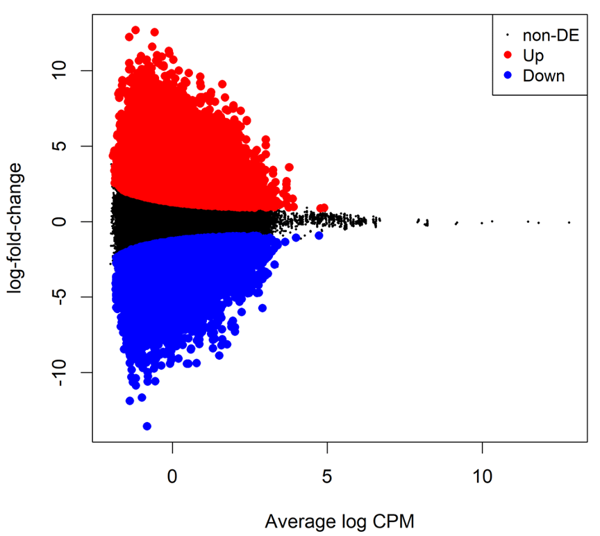
Comparing MethylKit and EdgeR


DAG of a complete DNA methylation data analysis pipeline

Reach Us!

Bioinformatics, Core Facility

Clinical Genomics Linköping